Welcome to part II in the series Machine Learning for Actuaries. In part I, we covered how to understand the General Problem Settings in Machine Learning. We also talked about what the Hypothesis Set is. For the sake of this blog, we will consider decision trees (all possible decision trees) as our hypothesis set.

We will cover how decision trees work and see a working example to implement decision trees in R. Please access it from the link below.

---

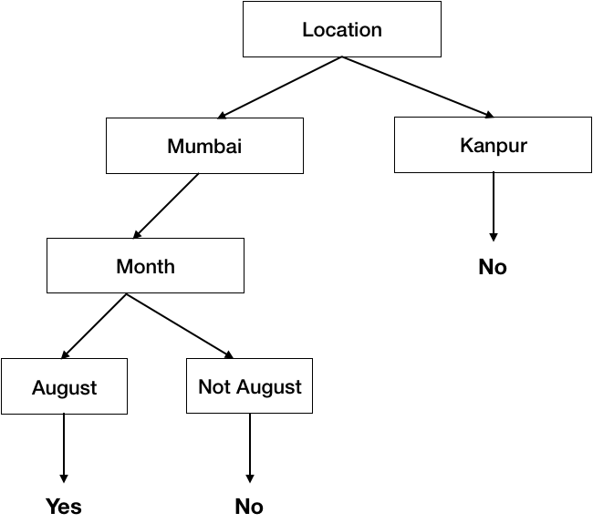
You use decision trees in a way in your life all the time, but very basic ones. Let’s say you stay in Mumbai, its August and you are going out, you would have to decide whether to take your umbrella with you or not because it might rain. Any Mumbaikar would suggest that you should carry an umbrella during August. But say you are just visiting Mumbai and you do not have any idea, what would you do? It is a typical decision tree problem statement. Let’s formulate this problem in a mathematical statement:

Let’s say you have < Location, Month, Temperature> as covariates to decide whether to take an umbrella with you or not and the response variable is “Take Umbrella”. What we want to do is to approximate a function f such that:

                *f* : < Location, Month, Temperature> → Take Umbrella

based on the data collected from people living in Mumbai and Delhi. We will get into that process of making decision trees later. But let’s look at what the output will look like.

---

Terminology related to Decision Trees:

Let’s look at the basic terminology used with Decision trees:
ROOT Node: It represents the entire population or sample and this further gets divided into two or more homogeneous sets.
SPLITTING: It is a process of dividing a node into two or more sub-nodes.
Decision Node: When a sub-node splits into further sub-nodes, then it is called a decision node.
Leaf/ Terminal Node: Nodes do not split is called Leaf or Terminal node.

In the above example:

• Each Internal Node (Boxes) tests 1 attribute of the data point (xi)
• Each Branch Node (Arrows) selects 1 value of data point (xi)
• Each Leaf Node (Bottom most arrows in Tree) predicts Output (Y)

---

Problem Setting would be:

Set of possible instances of X

• Each instance x in X is a feature vector of <Location, Month, Temperature> Unknown Target function f: X → Y
• Y is discrete valued ( ‘Yes’ or ‘No’) Set of function Hypothesis H = {h|h: X → Y}
• each hypothesis (h) in the Hypothesis set (H) is a decision tree
• trees sort X to leaf, which assigns the value to Y.

Note: We cannot use Decision Trees in the form described here to predict the continuous target variables. In order to do so, we have to alter the algorithm.

---

Top-Down method of making decision trees

Now that you have understood the decision trees and we have written our problem statement in the form of Problem Setting for machine learning, Let’s talk about how can we build an algorithm for decision trees?

node = Root Main Loop:

1. Select an attribute ‘A’ (the best decision attribute for the next node)
2. Assign ‘A’ as a decision attribute for the node
3. For each value of A create a new descendant of Node
4. Sort training examples to leaf nodes
5. If training examples can be perfectly classified at this leaf node, then stop, else go to the new leaf nodes created and consider them node and repeat the steps till you get perfect classification on all leaf nodes.

Question 1: Which attribute is the best? To answer that, let’s take an illustration. Suppose we have a dataset where the Target variable takes ‘Yes’ 29 times and ‘No’ 35 times. We can either split on attribute A1 or A2. The node looks like as in the image:

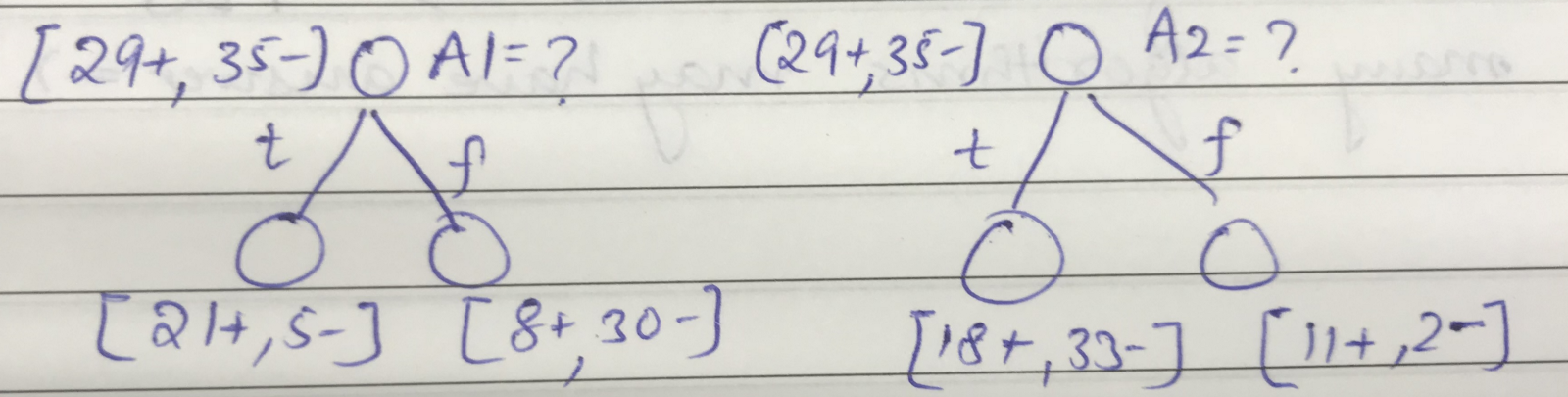
So A1 attribute creates 2 leaf nodes- Leaf Node 1 has classified most of the examples as positive and 5 negatives (No) and Leaf Node 2 has done the same thing, classified most examples as negative and a few as positives.

On the other hand A2 attribute’s 2 leaf nodes- Leaf node 2 has classified mostly but Leaf Node 1 has proportionated +ve and negatives, hence not a very useful Node.

A1 attribute is doing a better job than A2. Although the second decision tree might be able to classify the Target function very well once split on any other attribute, on the current stage A1 attribute is performing better. What we did is Greedily selected the attribute which makes the better split or more Homogeneous Leaf Node (Homogeneous is the exact term used). Thus, Decision Trees are known as greedy algorithms for classification.

Now you would say that it is easy for a human to recognize if the leaf node is Homogeneous, but how will computer get to know this? That leads to my next question

Question 2: How to define “Homogeneity” mathematically? Define a statistic to give information on how Homogeneous the data is?

The answer is Entropy.  The Entropy of a random variable is defined as :

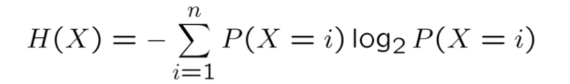
where n is all possible values of X.